Probabilistic Inference!!!

Assume we are given some dataset X with n features or variables and N number of data points. Letters in bold (x) denote vectors and the others are scalars.

This post considers only the approximate inference algorithms that are based on optimization.This is only an overview of such algorithms.

Learning the model of the data

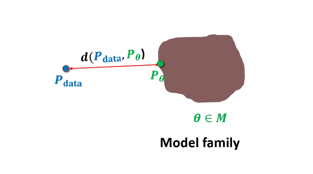
Learning involves estimating the underlying data distribution $p(\bf x)$.We assume the observed variable x is a random sample from an unknown underlying process, whose true distribution is unknown. We try to approximate the underlying process with a chosen model $p_{\theta}(\bf x)$ with parameter $\theta$. So, learning implies learning the parameter $\theta$.$p_{\theta}(\bf x)$ should be sufficiently flexible to be able to adapt to the data. Let $M$ denote the parameter space.

Two of the most commonly used models are:

• AutoRegressive Models (Pixel CNN, Character RNN)
• Latent Variable Models (VAE, Normalizing flow models, GAN, Inverse Autoregressive Flows)

The optimization criteria for models may be Maximum Likelihood or ELBO (Evidence Lower Bound which is a lower bound of likelihood) depending on the tractability of the likelihood of a model. Both the criteria are outcomes of Kullback-Leibler Divergence and are likelihood based. Generative adversarial networks come under latent variable models but the optimization criteria here is likelihood-free.

AutoRegressive Models

These models assume some topological ordering of the variables of the data. Based on the ordering,the distribution $p_{\theta}(\bf x)$ is factorized into product of conditionals. Each conditional can be parameterized separately.Let $\bf x_{< i}$ denote variables till i $(x_1,x_2,\dots,x_{i-1})$. If the order is assumed as sequential,then the model is factorized as $$p_{\theta}(\bf x)=\Pi_{i=1}^{n}p_{\theta}(x_i\vert \bf x_{< i})$$

For example consider the case of MNIST dataset. Each image can be considered as a 784 dimensional vector unrolled from left to right and top to bottom. AutoRegressive models can be used to generate one pixel based on the previously generated pixels (sequential ordering assumption).

Latent Variable Models

Latent variables are variables that are part of the model, but which we don’t observe. Latent variables are denoted by z and the model would then become $p_{\theta}(\bf x,\bf z)$. If the distributions are parameterized by neural networks, they are called Deep Latent Variable Models(DLVM).

Advantage of z

The marginal distribution over the datapoints $p_{\theta}(\bf x)$ is given by $$p_{\theta}(\bf{x}) = \int p_{\theta}(\bf x,\bf z)dz $$

This implicit distribution over x can be quite flexible. If z is discrete and $p_{\theta}(\bf{x} \vert \bf{z})$ is a Gaussian distribution,then $p_{\theta}(\bf x)$ is a mixture of Gaussian distributions. For continuous z, it can be seen as an infinite mixture of Gaussian distributions. The simplest and most common latent variable model is factorized as $$p_{\theta}(\bf{x}, \bf{z}) = p_{\theta}(\bf{z})p_{\theta}(\bf{x} \vert \bf{z}) $$

The distribution $p(\bf{z})$ is called as prior distribution over z.

Comments on the tractability of Likelihood

Learning the parameters requires the computation of likelihood for maximum likelihood learning. Gradient Descent algorithms are then used for finding the parameters that maximize the likelihood.

• Autoregressive models provide tractable likelihoods but no direct mechanism for learning features. They doesn’t learn any hidden representations or features like the latent variable models.
• Latent variable models can learn feature representations (via latent variables z) but have intractable marginal likelihoods because of the integral which is difficult to evaluate.

  Thats the reason why VAE’s approximate the posterior distribution $p_{\theta}(\bf{z} \vert \bf{x})$ and use ELBO which is a lower bound on the log-likelihood as the optimization criteria.GAN’s on the other hand don’t use likelihood as a criterion for optimization(doesn’t depend on likelihood directly).

• Latent Variable models that consists of flows like Normalizing Flow models have tractable likelihoods.

Written on August 12, 2018