The Gaussian!!

The Trivial Intro

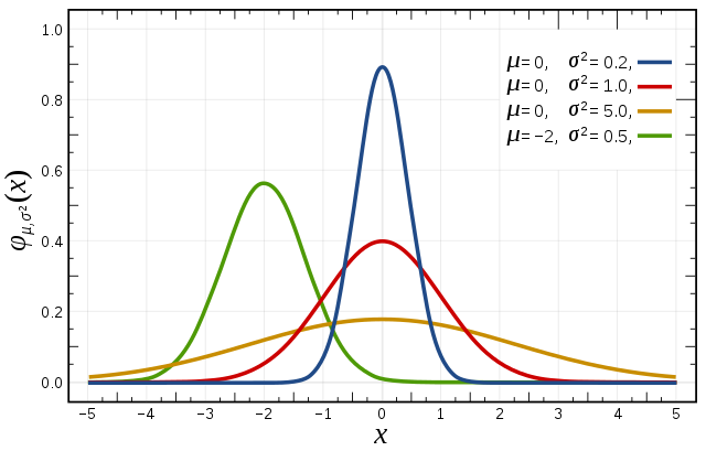
The Gaussian distribution is one of the most widely used continuous distribution with applications in many fields. It has several other names like normal distribution, bell curve. The density function with mean $\mu$ and variance $\sigma^2$ is given by: $$ f(x\vert \mu,\sigma^2)= \frac{1}{\sqrt{2\pi \sigma^2}}\exp^{\frac{-(x-\mu)^2}{2\sigma^2}} $$

The Chronicles of Gaussian

• Abraham de Moivre, an 18th-century statistician and consultant to gamblers, first discovered this distribution as an approximation to the binomial distribution. He observed that binomial distribution with a large number of trials approached a symmetric curve which he named it as normal curve.
• One of the first applications to normal distributions was made by Galileo for errors in astronomical observations. He observed that the errors were symmetric and that small errors occurred more frequently than large errors (distributions of many natural phenomena are at least approximately normally distributed).
• Later in the 18th century, Adrain and Gauss Independently developed the formula for the normal distribution and showed that errors were fit well by this distribution.
• The same distribution was discovered by Laplace when he derived the Central Limit Theorem which is considered to be one of the most important results in the theory of probability.

The Central Limit Theorem (The selling point of Gaussian )

In most of the stochastic or random models, mean/expectation is involved in one or the other ways. This is because, mean is the primary choice (others include median, mode) for a central measure of a distribution. The Central limit theorem connects the mean of any unknown distribution to the Gaussian.

We’ll go through the theorem using an interactive simulation for making it easy to grasp. First, we’ll look at the theorem statement in simple terms according to Wiki:

In probability theory, the central limit theorem (CLT) establishes that, in some situations, when independent random variables are added, their properly normalized sum tends toward a normal distribution (informally a “bell curve”) even if the original variables themselves are not normally distributed. The theorem is a key (“central”) concept in probability theory because it implies that probabilistic and statistical methods that work for normal distributions can be applicable to many problems involving other types of distributions.

So, when we are trying to estimate the mean of an unknown distribution through repeated sampling. CLT says that the probability distribution of the mean estimate tends to normal distribution as the sample size increases. This is true even-though the unknown distribution is not a normal distribution with the only condition that the variance of the unknown distribution should be finite.

Live Example

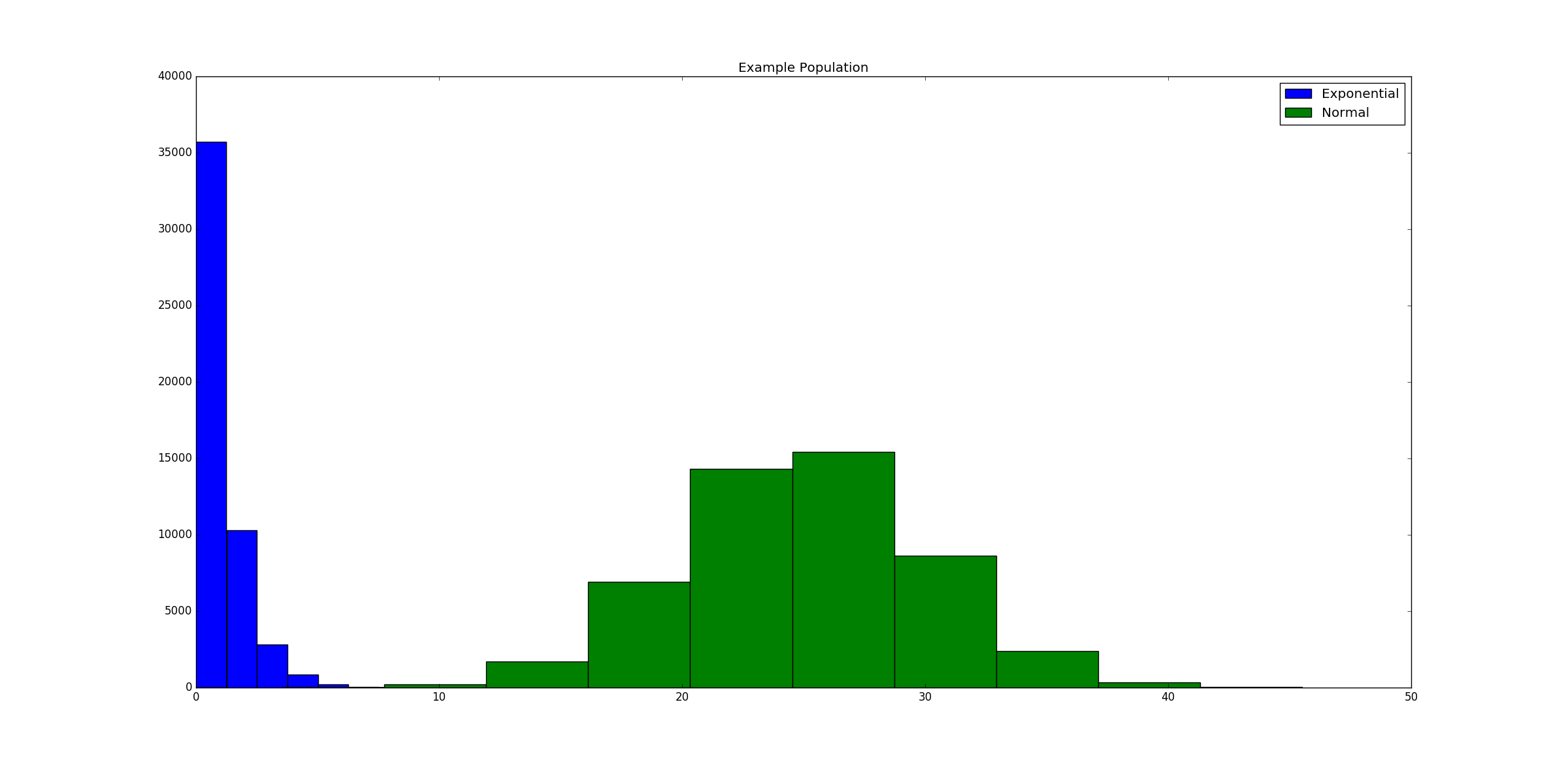
For example, let us take a population distribution as given below. The below-shown population consists of 100,000 numbers out of which half are sampled from the exponential distribution(parameter=1) and the other half from the normal distribution(mean=25,variance=5)

Now given a sample size s and the number of trials t, we sample (with replacement) s numbers from the population for t times. Mean of the samples for each time is recorded. This would be the sampling distribution of the mean of the population. The below code makes the things clear:

sample_sizes=[1,100,150,200,250]
trials=[100,500,2000]
data={}
for s in sample_sizes:
    for t in trials:
        mean=[]
        for k in range(t):
            sample=np.random.choice(population,size=s,replace=True)
            mean.append(np.mean(sample))
        data[str(s)+'_'+str(t)]=mean

Given below is an interactive plot of each setting. We can observe that as the sample size increases and if the number of trials are significant, the sampling distribution of the population mean estimate approaches the normal distribution.

Written on November 2, 2018